Snakemake for CMS Analysis Tutorial: All in One View

Content from The Why: Analysis Reproducibility

Last updated on 2026-02-08 | Edit this page

Estimated time: 10 minutes

Overview

Questions

Why do we need workflow orchestration in CMS?
What are the three pillars of a reusable analysis?
Who is the primary beneficiary of a reproducible workflow?

Objectives

Identify the “Knowledge Gap” in traditional HEP analyses.
Understand the three-step approach to capturing an analysis.
Recognize that reproducibility is a labor-saving tool for the analyst, not just a bureaucratic requirement.

The “Bus Factor” in CMS Analysis

In a typical CMS analysis, we move through Data Exploration, Background Modeling, Systematics, and Statistical Fits. Usually, this is handled by a series of disconnected scripts and manual steps.

The problem arises when an analyst moves on or a “Future You” returns to the code six months later:

The Environment: What version of CMSSW or Coffea was used?
The Logic: Why was this specific histogram used as input for that fit?
The Commands: What were the exact arguments passed to the script?

Without a workflow manager, this knowledge is lost, leading to “Scientific Archeology” where we try to dig up our own results.

The Three Pillars of Reusability

To solve this, we think of an analysis in three layers of “Capturing”:

Capture Code & Environment: Use Git for code and Containers (Docker/Apptainer) or Pixi/Conda for the software. This ensures the “Kitchen” is always the same.
Capture Commands: Move away from manual terminal commands. Use a script or a rule that explicitly states how to run the code.
Capture Workflow: This is the “Glue.” We define the relationship between steps. This is where Snakemake comes in.

Why should you care?

You might think: “Reproducibility is for the collaboration, but I’m just trying to graduate.”

Actually, the first person to benefit from a reproducible workflow is you.

The “Re-discovery” Phase: During the CMS review process (ARC), you will inevitably be asked to change a systematic or re-run a plot with new data. A Snakemake workflow allows you to do this by changing one line and typing one command.
Automation: Instead of waiting for Step A to finish so you can manually start Step B, you can launch the whole chain and go get coffee.

Challenge

Who is the most frequent user of your analysis code?

Show me the solution

Future You. Six months from now, when you have to re-run your plots for a conference or a paper revision, you will thank “Past You” for writing a Snakefile instead of a 20-page README.

Key Points

Modern CMS analysis is too complex to be managed by memory or manual scripts.
Reproducibility is a productivity tool: it makes your own work easier to revise and update.
Capturing the Workflow (the “Glue”) is the final step in ensuring an analysis is truly reusable.

Content from Introduction to Snakemake

Last updated on 2026-02-17 | Edit this page

Estimated time: 20 minutes

Overview

Questions

What is a Snakefile?
How do I define a single processing step?
How do I execute a rule?

Objectives

Create a Snakefile.
Write a valid Snakemake rule with input, output, and shell.
Execute a specific target file.

Snakemake Logo

Why Snakemake for CMS?

In CMS analysis, we rarely run a single script. We create an analysis chain: Skimming \(\rightarrow\) Processing \(\rightarrow\) Plotting \(\rightarrow\) Fitting. Traditionally, we managed this with “Mega-Bash” scripts or by manually submitting JDL files to HTCondor/Slurm.

Key Advantages

Portability: Works on your laptop, LXPLUS, or the LPC with the same code.
Environment Management: Seamless integration with Containers (Apptainer/Singularity) and Conda.
Visualization: It automatically generates a “map” (Directed Acyclic Graph or DAG) of your analysis.

Snakemake vs. LAW (Luigi Analysis Workflow): A bias comparison

Boilerplate: LAW is based on Luigi and requires significant Python boilerplate for every task. Snakemake uses a “Domain Specific Language” (DSL) that is much closer to plain English or a configuration file.
The Learning Curve: Snakemake is widely used in Genomics and Data Science. If you search for a problem on StackOverflow, you’ll find an answer in seconds. LAW is more niche to the HEP community.
Automation: Snakemake is file-based. It looks at the “last modified” timestamp of your files. If you change your plotting script, it won’t re-run the 5-hour skimming step unless you ask it to.
Workflow Isolation: All your code can run independently of Snakemake. You can think of Snakemake as a “workflow manager” that orchestrates your existing scripts (like a bash script on steroids). LAW requires you to write your tasks as Luigi Tasks, which can be more cumbersome.

Callout

Credits and Documentation

Snakemake is an open-source project created by Johannes Köster (University of Duisburg-Essen) in 2012. While this tutorial focuses on CMS-specific use cases, the official documentation is comprehensive and covers thousands of features.

Documentation: https://snakemake.github.io
Citation: If you use Snakemake in your analysis, proper citation is expected in our field:

Köster, Johannes and Rahmann, Sven. “Snakemake—a scalable bioinformatics workflow engine”. Bioinformatics, 2012.

The Essentials

To run a workflow, you need two things:

The Snakefile: A file named Snakefile (capital S, no extension) where you define your rules. It uses a Python-based syntax, so you can write standard Python code inside it alongside your rules.
The Execution Command: You run the workflow from the terminal by invoking snakemake.

The basic command structure is:

BASH

snakemake --cores <N> <target_file>

--cores <N>: Tells Snakemake how many CPU cores to use. (e.g., --cores 1 for sequential execution, --cores 4 for parallel).
<target_file>: The file you want to generate. Snakemake will figure out the steps to get there.
If you dont specify a snakefile, Snakemake will look for a file named Snakefile in the current directory. You can specify a different file with -s <filename>.

The Anatomy of a Rule

The building block of Snakemake is the rule. Think of it as a recipe. To make a dish, you need ingredients (inputs), a kitchen (the environment), and a set of instructions (the shell command).

PYTHON

rule skim_data:
    input:
        "raw_data.txt"
    output:
        "skimmed_data.txt"
    shell:
        "grep 'Signal' {input} > {output}"

Important Properties:

Rule Name: Must be unique.
Input/Output: These are strings (or lists of strings). Snakemake uses these to “connect the dots” between rules.
Shell: The bash command to execute. Notice the {input} and {output} placeholders—Snakemake automatically fills these in with the paths you defined above.

Understanding the Syntax

A Snakefile is essentially a Python script with some extra keywords added. This is powerful because it means you can use Python variables, functions, and libraries directly in your workflow definition.

Indentation matters: Just like in Python, Snakemake uses indentation (usually 4 spaces) to group code blocks. The input, output, and shell directives must be indented relative to the rule.
Strings: File paths and commands are strings, so they must be enclosed in quotes ("..." or '...').
Comments: Use # for comments, just like in Python/Bash.
Lists: If a rule has multiple inputs or outputs, you can list them with commas:

PYTHON

    input:
        "file1.txt",
        "file2.txt"

Running the Rule

Create dummy data:

BASH

echo -e "Background\nSignal\nBackground\nSignal" > raw_data.txt

Create a Snakefile with the content shown above.
Run Snakemake. We must tell it what file we want to generate:

BASH

pixi run snakemake --cores 1 skimmed_data.txt
# if you run snakemake from a conda environment or pip, use:
# snakemake --cores 1 skimmed_data.txt

If successful, you will see Finished jobid: 0.

Output

OUTPUT

Assuming unrestricted shared filesystem usage.
host: gluon
Building DAG of jobs...
Using shell: /usr/bin/bash
Provided cores: 1 (use --cores to define parallelism)
Rules claiming more threads will be scaled down.
Job stats:
job          count
---------  -------
skim_data        1
total            1

Select jobs to execute...
Execute 1 jobs...

[Sun Feb  8 12:05:08 2026]
localrule skim_data:
    input: raw_data.txt
    output: skimmed_data.txt
    jobid: 0
    reason: Missing output files: skimmed_data.txt
    resources: tmpdir=/tmp
[Sun Feb  8 12:05:08 2026]
Finished jobid: 0 (Rule: skim_data)
1 of 1 steps (100%) done

Instructor Note

If snakemake was not installed using pixi but with a conda environment or pip, you should remove the pixi run part and just run:

BASH

snakemake --cores 1 counts.txt

This will be the case for most users following this tutorial outside of the pixi environment.

Challenge

Syntax Error Hunt

Intentionally break your indentation (remove a space before input:). Run the command again.

What error does Snakemake give you?

Show me the solution

This IndentationError is the most common error you will encounter.

Key Points

A Snakefile defines the workflow.
A rule contains input, output, and a shell command.
You execute the workflow by asking for the output file, not the rule name.

Content from Chaining Rules (The DAG)

Last updated on 2026-02-17 | Edit this page

Estimated time: 30 minutes

Overview

Questions

How does Snakemake connect different rules?
What is a DAG?
How does Snakemake know what to re-run?

Objectives

Connect two rules by matching input/output filenames.
Use the rule all convention.
Observe “Lazy Execution” in action.

Thinking Backwards

The most difficult paradigm shift when learning Snakemake is that you stop writing Imperative instructions (Step A, then Step B) and start writing Declarative goals.

In a Bash script, you say: > “Run the skimmer. Then run the plotter.”

In Snakemake, you say: > “I want the plot. To get the plot, I need the skimmed file. To get the skimmed file, I need the raw data.”

Snakemake determines the dependencies automatically by matching filenames. If Rule A outputs file.txt and Rule B takes file.txt as input, Snakemake knows Rule A must run first. This chain of dependencies is called a DAG (Directed Acyclic Graph).

Activity: Extending the Analysis

We have a rule that skims data. Now we want to count the events in that skimmed file.

Add this second rule to your Snakefile (below the first one):

PYTHON

rule count_events:
    input:
        "skimmed_data.txt" 
    output:
        "counts.txt"
    shell:
        "wc -l {input} > {output}"

Crucial Link: Notice that the input of count_events matches the output of skim_data. This is how Snakemake builds the Directed Acyclic Graph (DAG).

Running the Chain

Ask for the final result:

BASH

pixi run snakemake --cores 1 counts.txt

Snakemake realizes:

You want counts.txt.
count_events can produce it, but it needs skimmed_data.txt.
skim_data can produce skimmed_data.txt. Plan: Run skim_data -> Run count_events.

The rule all Convention

By default, Snakemake runs the first rule it sees if you don’t specify a file. To avoid typing counts.txt every time, we add a “dummy” rule at the very top.

Add this to the top of your Snakefile:

PYTHON

rule all:
    input:
        "counts.txt"

Now you can simply run:

BASH

pixi run snakemake --cores 1

Challenge

Lazy Execution (The “Why”)

Run pixi run snakemake --cores 1 again.

What happens?

OUTPUT

Assuming unrestricted shared filesystem usage.
host: xxxx
Building DAG of jobs...
Nothing to be done (all requested files are present and up to date).

Modify the original raw data:

BASH

touch raw_data.txt

For MacOS users: some students have reported that touch does not remove the timestamp. In this case, you can remove the file and re-create it, or try to change the content.

Run Snakemake again.

What happens?

Show me the solution

When you first run the command, Snakemake checks if counts.txt exists. Since it doesn’t, it calculates the steps needed to create it. The second time you run the command, Snakemake sees that counts.txt exists and is newer than its inputs, so it does nothing.

When you “touch” raw_data.txt, you update its modification time. Snakemake notices that an input (raw_data.txt) is now strictly newer than the downstream files (skimmed_data.txt and counts.txt). It marks them as “stale” and re-runs the chain.

This is the crucial benefit for large analyses. If you had a workflow with 500 rules and you only modified the input for rule 499, Snakemake would not re-run rules 1 through 498. It selectively re-executes only the parts of the DAG that are affected by your change. In CMS terms: if you change a plotting style, you don’t have to re-run the N-tuplizer.

Key Points

Declarative Workflows: Unlike bash scripts where you define the order of steps, in Snakemake you define the dependencies (inputs/outputs), and Snakemake figures out the order (DAG).
The all Rule: It is convention to include a rule named all at the top of the workflow to define the final targets of your analysis.
Lazy Execution: Snakemake only re-runs a rule if the output file is missing or if the input files have changed (have a newer timestamp) since the last run.

Content from Scaling with Wildcards

Last updated on 2026-02-08 | Edit this page

Estimated time: 30 minutes

Overview

Questions

How can I use one rule to process multiple different samples?
What is a wildcard and how does Snakemake “fill” it?
How do I tell Snakemake to generate a list of all my target files?

Objectives

Replace hardcoded filenames with {wildcards}.
Use the expand() function to generate lists of outputs.
Understand how Snakemake “pattern matches” files on disk.

Scaling Up: From One File to Many

In CMS, we never have just one “raw_data.txt”. We have DYJets, TTbar, WJets, and various Data eras. Writing a rule for each one would be a nightmare.

Snakemake handles this using Wildcards.

The Wildcard Syntax

A wildcard is a placeholder in curly braces {}. For example, instead of writing a rule that only processes TTbar.txt, we can write a generic rule that works for any sample:

PYTHON

rule skim_data:
    input:
        "raw/{sample}.txt"
    output:
        "skimmed/{sample}.txt"
    shell:
        "grep 'Signal' {input} > {output}"

How does it work?

When you ask for skimmed/TTbar.txt, Snakemake looks at the rule and sees it can create skimmed/{sample}.txt. It “pattern matches” and determines that {sample} must be TTbar. It then looks for the input TTbar.txt.

Crucial Rule: Snakemake works backwards. It looks at the output you requested, matches it to the output pattern of a rule, determines the wildcard value, and then fills in that value for the input.

The `expand()` function

If you have 100 samples, you don’t want to type them all in your rule all. Snakemake provides a helper function called expand() to generate lists of files.

PYTHON

SAMPLES = ["DYJets", "TTbar", "WJets"]

rule all:
    input:
        expand("skimmed/{s}.txt", s=SAMPLES)

The expand() function takes a pattern and replaces the placeholders with the values in your list. The code above produces: ["skimmed/DYJets.txt", "skimmed/TTbar.txt", "skimmed/WJets.txt"]

Callout

Wildcards vs. Expand Variables

Notice a subtle difference:

In rule skim_data, we used {sample}. This is a Wildcard (Snakemake figures it out based on the filename).
In rule all, we used {s} inside expand(). This is a Python string formatting variable.

They do not need to match! expand() happens before the rules run to generate the list of target files. The rules run after to figure out how to create those files.

Activity: Processing Multiple Datasets

Instructor Note

Parallelism: This is the best moment to explain why the --cores flag matters. In HEP, we are used to sending 100 jobs to Condor. Here, we show they can run 4 (or 8, or 16) jobs in parallel locally on their laptop with zero extra effort.
The “Pattern Matching” Warning: Students often try to put wildcards in the input that aren’t in the output. I would emphasize that Snakemake works backwards: it sees a file it wants (the output) and then tries to figure out what the input should be.

Let’s modify our Snakefile to handle three different simulated datasets.

Open your Snakefile and modify it as follows:

PYTHON

# 1. Define our datasets
DATASETS = ["DYJets", "TTbar", "Data"]

rule all:
    input:
        expand("results/{d}_counts.txt", d=DATASETS)

# 2. Updated Skim rule with wildcards
rule skim_data:
    input:
        "raw/{dataset}.txt"
    output:
        "skimmed/{dataset}.txt"
    shell:
        "grep 'Signal' {input} > {output} || true"

# 3. Updated Count rule with wildcards
rule count_events:
    input:
        "skimmed/{dataset}.txt"
    output:
        "results/{dataset}_counts.txt"
    shell:
        "wc -l {input} > {output}"

Prepare the “raw” directory and files:

BASH

mkdir -p raw
echo -e "Signal\nBackground" > raw/DYJets.txt
echo -e "Signal\nSignal\nBackground" > raw/TTbar.txt
echo -e "Background\nBackground" > raw/Data.txt

Run the workflow. Note that we use –cores 4 to allow Snakemake to run independent jobs in parallel:

BASH

pixi run snakemake --cores 4

Challenge

Exercise: Adding a new sample

Add a new dataset called WJets to your DATASETS list.

Create the dummy file raw/WJets.txt with some “Signal” lines.
Run Snakemake again.

Show me the solution

Observe how Snakemake only runs the rules for the new WJets sample and skips the ones that were already finished (DYJets, TTbar, Data).

Key Points

Wildcards: Use name in filenames to define a generic rule.
Constraints: Snakemake fills wildcards by looking at the output you requested and propagating that value to the input.
expand(): A Python function that generates a list of filenames from a pattern. It is commonly used in rule all to define the final targets.
Parallelism: With wildcards, Snakemake can run multiple independent jobs in parallel using the --cores flag.

Content from Visualizing the Workflow

Last updated on 2026-02-17 | Edit this page

Estimated time: 20 minutes

Overview

Questions

How can I see the dependencies between my rules?
What is a Directed Acyclic Graph (DAG)?
How do I preview what Snakemake intends to do?

Objectives

Use the --dag flag to generate a visualization of the analysis.
Understand the difference between the Rule Graph and the File Graph.
Use dry-runs (-n) to verify the execution plan.

Seeing the Big Picture

As your analysis grows from 2 rules to 20, and from 3 samples to 300, it becomes impossible to keep the entire workflow in your head. Snakemake provides built-in tools to “draw” your analysis for you.

The Directed Acyclic Graph (DAG)

Snakemake represents your workflow as a DAG:

Directed: There is a clear flow from raw data to final plots.
Acyclic: There are no loops (you can’t have a file that depends on its own output).
Graph: A mathematical structure of nodes (rules/files) and edges (dependencies).

Generating the DAG

To create a visualization, we tell Snakemake to generate the DAG in a format called dot, and then we use the graphviz tool (which we installed via pixi in the setup) to turn it into an image.

BASH

pixi run snakemake --dag | dot -Tpng > dag.png
# pixi run snakemake --dag | dot -Tpdf > dag.pdf   ### For PDF format

How to read the DAG:

Nodes (Boxes): Represent the jobs that need to be run.
Arrows: Represent the flow of data.
Solid vs. Dashed lines: In many viewers, a dashed border indicates that the file already exists and the job doesn’t need to run.

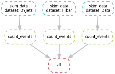
Activity: Visualizing our Scaled Workflow

Ensure you have the Snakefile from the previous episode (with DYJets, TTbar, Data, and WJets).
Run the DAG command:

BASH

pixi run snakemake --dag | dot -Tpng > dag.png

For MacOS users

It has been reported that the command above may not work due to differences in how dot is handled. If you encounter issues, try the following command instead:

BASH

pixi run snakemake --dag | pixi run dot -Tpng > dag.png

or you can run:

BASH

pixi run dot -C
pixi run snakemake --dag | pixi run dot -Tpng > dag.png

Open dag.png, it should look like the following image. Notice how the branches for each dataset are parallel.

Challenge

Exercise: Identifying the Bottleneck

Look at your DAG. If you were to run this on a machine with only 1 core, how many steps would it take? If you had 4 cores, how would the timing change?

Show me the solution

With 1 core, Snakemake runs every job sequentially. With 4 cores, Snakemake can run all four skim_data jobs simultaneously, significantly reducing the “Wall Clock” time of your analysis. This is the power of a DAG-based system!

Callout

Rule Graph vs. File Graph

If you have 1,000 samples, the --dag command will produce a giant PDF with 1,000 boxes, which is unreadable. To see a simplified version that only shows how the rules connect (ignoring the individual samples), use:

BASH

pixi run snakemake --rulegraph | dot -Tpng > rulegraph.png

This is often much more useful for complex CMS analyses to ensure the logic is correct.

The Dry-Run: “Look Before You Leap”

Before you submit 1,000 jobs to a cluster, you should always perform a Dry-Run. This tells Snakemake to calculate the DAG and print the execution plan without actually running any commands.

BASH

pixi run snakemake -n

If you want more detail (like seeing the actual shell commands that will be executed), use:

BASH

pixi run snakemake -n -p

Did the previous command work?

If you run this commands on top of finished workflow, you should see something like:

OUTPUT

Building DAG of jobs...
Nothing to be done (all requested files are present and up to date).

This is expected, because all the output files already exist. If you change something in your Snakefile (like adding a new rule or changing an existing one), the dry-run will show you which jobs need to be re-run.

Alternatively, if you want to see the dry-run or the commands to execute, use:

BASH

pixi run snakemake -n -p --forceall

Key Points

DAG: A visual map of your analysis dependencies.
Dry-run (-n): Always perform a dry-run to verify the plan before executing.
Rule Graph: A simplified visualization showing the relationship between rules rather than individual files.

Content from Containerized Execution

Last updated on 2026-02-16 | Edit this page

Estimated time: 30 minutes

Overview

Questions

How do I run specific steps of my analysis in a controlled environment?
How can I use CMSSW or specific Python versions without installing them locally?
How does Snakemake handle Apptainer/Singularity?

Objectives

Use the container: directive to link a rule to a Docker/Apptainer image.
Execute a workflow where different rules use different environments.
Understand the --use-apptainer (or --use-singularity) flag.

Containers: Your Analysis in a Box

In CMS, we often need very specific environments: a certain version of CMSSW, a specific ROOT version for combine, or a set of Python libraries like coffea. Instead of spending hours fighting with export PATH or cmsenv, we can use Containers.

Snakemake makes this seamless. You can tell a specific rule to run inside a container, and Snakemake will automatically pull the image and wrap your command inside it.

My Opinions on this Episode

The “LPC/LXPLUS” connection: This is where you should mention that on most HEP clusters, singularity or apptainer is already installed. This makes their local tutorial 100% transferable to the big machines.
Binding directories: Students often ask how the container sees their files. It’s worth a small note that Snakemake automatically “binds” the project directory so the container sees the code and data.

The `container:` Directive

To use a container, you simply add the container: keyword to your rule.

PYTHON

rule plot_data:
    input:
        "results/{dataset}_counts.txt"
    output:
        "plots/{dataset}.png"
    container:
        "docker://python:3.10-slim"
    shell:
        "python scripts/my_plotter.py {input} {output}"

What happens behind the scenes?

When you run Snakemake with the --use-apptainer flag:

Snakemake sees the container: directive.
It pulls the image (if not already present) using Apptainer/Singularity. Note: Apptainer can run docker:// images perfectly fine.
It starts the container and automatically mounts (binds) your current working directory inside it.
It executes the shell command inside that container.

Why is this better than a local environment?

Portability: You can run the exact same container on your laptop, the LPC, or the Grid.
Isolation: Rule A can use python:2.7 while Rule B uses python:3.11. No more version conflicts!
No Installation: You don’t need to install ROOT or CMSSW on your machine; you just need to point to the image.

Callout

A Note on Apptainer Installation

While we are using Pixi to manage Snakemake and our local Python tools, Pixi does not typically install Apptainer/Singularity itself. This is because Apptainer requires specific system-level permissions to manage containers safely.

On your laptop: You must have Apptainer installed at the system level (e.g., via brew on macOS with a virtual machine, or your Linux distribution’s package manager).
On CMS Clusters (LPC/LXPLUS): Apptainer is already pre-installed by the administrators.

Before proceeding, verify you have it by running: apptainer --version.

Activity: Running a “Physics” Script in a Container

Let’s simulate a plotting step that requires a specific Python environment.

Create a simple plotting script named plotter.py:

PYTHON

import sys
# Simulate a plotting library requirement
print(f"Generating plot from {sys.argv[1]} using Python {sys.version}")
with open(sys.argv[2], "w") as f:
    f.write("IMAGE_DATA")

Modify your Snakefile to include a containerized plotting rule:

PYTHON

DATASETS = ["DYJets", "TTbar", "Data"]

rule all:
    input:
        expand("plots/{d}.png", d=DATASETS)

# (Keep your previous skim_data and count_events rules here)

rule plot_results:
    input:
        "results/{dataset}_counts.txt"
    output:
        "plots/{dataset}.png"
    container:
        "docker://python:3.10-slim"
    shell:
        "python plotter.py {input} {output}"

Run the workflow using Apptainer:

BASH

pixi run snakemake --cores 1 --use-apptainer

Callout

Please note that the previous exercise will create empty “plots” since the plotter.py is just a placeholder. The point is to see the container in action, not to generate real plots!

Did it work? Depending on where you run it, this answer may vary. If you are running on lxplus/cmslpc, you might get an error about bindings or permissions. This is the next topic we’ll cover.

Accessing External Data (Bind Mounts)

By default, Snakemake only lets the container see files inside your current project folder.

The CMS Problem: In HEP, our data typically lives on storage areas like /eos or /cernbox, and our software might live on /cvmfs. If you try to access a file in /eos/user/... from inside the container, it will fail because the container is isolated.

The Solution: You can pass arguments to Apptainer using the --apptainer-args flag in Snakemake:

BASH

pixi run snakemake --cores 1 --use-apptainer --apptainer-args "--bind /eos:/eos --bind /cvmfs:/cvmfs"  ### --bind /uscms_data/d3/user/ if you are at the LPC

This tells Apptainer: “Poke a hole in the container so I can see /eos and /cvmfs from the outside.”

Challenge

Exercise: Different Containers for Different Tasks

Imagine your skim_data rule requires an old C++ library only available in a cmssw image, but your plot_results rule needs a modern coffea environment.

Can you assign different container: directives to different rules in the same Snakefile?
Try changing the container: in plot_results to docker://alpine:latest and run it. What happens?

Show me the solution

Yes! Snakemake is designed for this. It will start the correct container for each specific job. If you switch to alpine:latest, the job will fail because alpine does not have python installed by default—this proves the command is truly running inside the isolated container!

Key Points

container:: A rule-level directive that specifies the Docker/Apptainer image to use.
–use-apptainer: The command-line flag required to enable container execution.
*–apptainer-args: Use this to bind external storage paths (like /eos or /cvmfs) so the container can see them.
Environment Agnostic: You can mix and match different containers in a single workflow, ensuring each step has the exact dependencies it needs.

Content from Bonus: The CMSDAS Challenge

Last updated on 2026-02-17 | Edit this page

Estimated time: 60 minutes

Overview

Questions

How do I integrate existing CMS analysis repositories into Snakemake?
How do I handle scripts that produce non-deterministic outputs (timestamps)?
How do I chain different software environments (Coffea \(\rightarrow\) Combine)?

Objectives

Clone and configure the \(t\bar{t}\gamma\) analysis repository.
Write a rule to parallelize the processing step.
“Patch” the aggregation step to accept Snakemake inputs.
Execute a final statistical fit using a dedicated combine container.

The Challenge: \(t\bar{t}\gamma\) Cross Section

In the previous episodes, we worked with toy scripts. Now, we will automate a real analysis: the CMSDAS \(t\bar{t}\gamma\) Long Exercise. For this tutorial, we are not interested about the physics details, but rather how to integrate an existing analysis workflow into Snakemake. If you want to know more about the physics, check the CMSDAS \(t\bar{t}\gamma\) Long Exercise repository.

This analysis has a typical structure:

Coffea Processor (runFullDataset.py): Runs on NanoAODs and produces .coffea histograms.
Plotting/Conversion (save_to_root.py): Aggregates histograms and saves them as .root files for the fit.
Statistics (combine): Performs a likelihood fit to extract the cross-section.

Setting the Stage

First, we need the analysis code. We will clone the repository directly into our workflow directory.

BASH

# Clone the repository (using the facilitators2026 branch for this tutorial)
git clone -b facilitators2026 https://github.com/fnallpc/ttgamma_longexercise.git

Now, check the contents. Notice that we are using the facilitators2026 branch (the solutions branch). You should see runFullDataset.py and a ttgamma/ directory.

Callout

Notice that we are trying to give a “realistic” experience in this tutorial. The code is not designed for Snakemake, so we will have to make some adjustments and “patches” to make it work. This is a common scenario when integrating legacy code into modern workflows.

Step 1: The processing Rule

Patch 1: Removing Timestamps from runFullDataset.py

Open ttgamma_longexercise/runFullDataset.py and scroll to the bottom. You will see lines that look like this:

PYTHON

    timestamp = datetime.datetime.now().strftime("%Y%m%d_%H%M%S")
    outfile = os.path.join(args.outdir, f"output_{args.mcGroup}_run{timestamp}.coffea")
    util.save(output, outfile)

The Problem: Snakemake relies on filenames to know if a job finished. If the script adds a random timestamp (e.g., _run20260215...), Snakemake won’t know the file was created, and the workflow will fail.

The Fix: Modify the code to remove the timestamp. Change those lines to:

PYTHON

    # timestamp = datetime.datetime.now().strftime("%Y%m%d_%H%M%S")
    # Remove the timestamp from the filename
    outfile = os.path.join(args.outdir, f"output_{args.mcGroup}.coffea")
    util.save(output, outfile)

Now the output is predictable: output_MCTTGamma.coffea.

We can write a clean Snakemake file with the following rules. We will define a rule that runs runFullDataset.py for each group (e.g., MCTTGamma, Data, etc.) and produces a .coffea file for each.

PYTHON

# Define the groups (found in runFullDataset.py)
MC_GROUPS = ["MCTTGamma", "MCTTbar1l", "MCTTbar2l", "MCSingleTop", "MCZJets", "MCWJets", "MCOther"]
DATA_GROUPS = ["Data"]
ALL_GROUPS = MC_GROUPS + DATA_GROUPS

rule run_coffea:
    input:
        script = "ttgamma_longexercise/runFullDataset.py"
    output:
        "results/output_{group}.coffea"
    container:
        #docker://coffeateam/coffea-dask-almalinux9:2025.9.0-py3.10"
        "/cvmfs/unpacked.cern.ch/registry.hub.docker.com/coffeateam/coffea-dask-almalinux9:2025.9.0-py3.10"   #### it can be from cvmfs
    shell:
        # We run with the modified script which outputs deterministic filenames
        "python {input.script} {wildcards.group} --outdir results --workers 1 --executor local --maxchunks 1"
        #"python {input.script} {wildcards.group} --outdir results --executor lpcjq"   ### if you want to run the full dataset, takes hours.

Step 2: The Aggregation Patch

The second step of the analysis is to aggregate the .coffea files and convert them to ROOT.

Patch 2: Enabling Arguments in save_to_root.py

The original script ttgamma_longexercise/save_to_root.py has a major issue for automation and we will modify it.

PYTHON

outputMC = accumulate(
    [
        util.load("results/output_MCOther.coffea"),
        util.load("results/output_MCSingleTop.coffea"),
        util.load("results/output_MCTTbar1l.coffea"),
        util.load("results/output_MCTTbar2l.coffea"),
        util.load("results/output_MCTTGamma.coffea"),
        util.load("results/output_MCWJets.coffea"),
        util.load("results/output_MCZJets.coffea"),
    ]
)

outputData = util.load("results/output_Data.coffea")

The second step of the analysis is to aggregate the .coffea files and convert them to ROOT. After you modify the code to remove the timestamp, we can write a Snakemake rule that depends on all the .coffea files and runs the aggregation script.

PYTHON

rule make_root_files:
    input:
        # 1. We need ALL the group files to be finished
        coffeas = expand("results/output_{group}.coffea", group=ALL_GROUPS),
        # 2. The script we just created
        script = "ttgamma_longexercise/save_to_root.py"
    output:
        # The file expected by the next step (Combine)
        "RootFiles/M3_Output.root"
    container:
        # We use the same container as the processing step
        #docker://coffeateam/coffea-dask-almalinux9:2025.9.0-py3.10"
        "/cvmfs/unpacked.cern.ch/registry.hub.docker.com/coffeateam/coffea-dask-almalinux9:2025.9.0-py3.10"   #### it can be from cvmfs
    shell:
        # Pass the output filename first, then all input files
        "python {input.script} {output} {input.coffeas}"

Step 3: The Fit (Hybrid Environments)

Now that we have ROOT files, we need to run combine. This requires a completely different environment (CMSSW-based).

While we usually use the container: directive, complex HEP software like CMSSW often requires sourcing environment scripts (/cvmfs/.../cmsset_default.sh) that don’t play nicely with the automatic entrypoints of some containers.

In these cases, it is safer to invoke apptainer explicitly inside the shell command.

PYTHON

rule run_combine:
    input:
        root_file = "RootFiles/M3_Output.root",
        # We use the data card from the repo
        card = "ttgamma_longexercise/Fitting/data_card.txt",
        #container = "docker://gitlab-registry.cern.ch/cms-cloud/combine-standalone:latest"
        container = '/cvmfs/unpacked.cern.ch/gitlab-registry.cern.ch/cms-analysis/general/combine-container:latest'
    output:
        "fitDiagnosticsTest.root"
    shell:
        """
        APPTAINER_SHELL=$(which bash) apptainer exec -B .:/home/cmsusr/analysis \
            -B /cvmfs --pwd /home/cmsusr/analysis/  \
            {input.container} \
                /bin/bash -c "export LANG=C && export LC_ALL=C && \
                source /cvmfs/cms.cern.ch/cmsset_default.sh && \
                cd /home/cmsusr/CMSSW_14_1_0_pre4/ && \
                 cmsenv && \
                 cd - && \
                text2workspace.py {input.card} -m 125 -o workspace.root && \
                combine -M FitDiagnostics workspace.root --saveShapes --saveWithUncertainties"
        """

The Grand Finale

Now, define your target in rule all.

PYTHON

rule all:
    input:
        "fitDiagnosticsTest.root"

Run it!

BASH

pixi run snakemake --cores 4 --use-apptainer

Callout

What just happened?

Snakemake saw you wanted the Fit.
It checked make_root_files, which needed the .coffea files.
It launched 8 parallel jobs to process Data, TTGamma, TTbar, etc., using the Coffea container.
Once all 8 finished, it ran the aggregation script.
Finally, it switched to the Combine container and performed the fit.

You have just orchestrated a full CMS analysis involving Data, MC, Systematics, and Statistics with one command.

Comparing Snakefile with a Bash Script

Let’s compare this with how you would do it in a bash script.

Full Snakefile for Reference

PYTHON

# Define the groups (found in runFullDataset.py)
MC_GROUPS = ["MCTTGamma", "MCTTbar1l", "MCTTbar2l", "MCSingleTop", "MCZJets", "MCWJets", "MCOther"]
DATA_GROUPS = ["Data"]
ALL_GROUPS = MC_GROUPS + DATA_GROUPS

rule all:
    input:
        #expand("results/output_{group}.coffea", group=ALL_GROUPS),
        #"RootFiles/M3_Output.root",
        "fitDiagnosticsTest.root"

rule run_coffea:
    input:
        script = "ttgamma_longexercise/runFullDataset.py"
    output:
        "results/output_{group}.coffea"
    container:
        #docker://coffeateam/coffea-dask-almalinux9:2025.9.0-py3.10"
        "/cvmfs/unpacked.cern.ch/registry.hub.docker.com/coffeateam/coffea-dask-almalinux9:2025.9.0-py3.10"   #### it can be from cvmfs
    shell:
        # We run with the modified script which outputs deterministic filenames
        "python {input.script} {wildcards.group} --outdir results --workers 1 --executor local --maxchunks 1"
        #"python {input.script} {wildcards.group} --outdir results --executor lpcjq"

rule make_root_files:
    input:
        # 1. We need ALL the group files to be finished
        coffeas = expand("results/output_{group}.coffea", group=ALL_GROUPS),
        # 2. The script we just created
        script = "ttgamma_longexercise/save_to_root.py"
    output:
        # The file expected by the next step (Combine)
        "RootFiles/M3_Output.root"
    container:
        # We use the same container as the processing step
        #docker://coffeateam/coffea-dask-almalinux9:2025.9.0-py3.10"
        "/cvmfs/unpacked.cern.ch/registry.hub.docker.com/coffeateam/coffea-dask-almalinux9:2025.9.0-py3.10"   #### it can be from cvmfs
    shell:
        # Pass the output filename first, then all input files
        "python {input.script} {output} {input.coffeas}"


rule run_combine:
    input:
        root_file = "RootFiles/M3_Output.root",
        # We use the data card from the repo
        card = "ttgamma_longexercise/Fitting/data_card.txt",
        #container = "docker://gitlab-registry.cern.ch/cms-cloud/combine-standalone:latest"
        container = '/cvmfs/unpacked.cern.ch/gitlab-registry.cern.ch/cms-analysis/general/combine-container:latest'
    output:
        "fitDiagnosticsTest.root"
    shell:
        """
        #export APPTAINER_CACHEDIR="/tmp/$(whoami)/apptainer_cache"
        #export APPTAINER_TMPDIR="/tmp/.apptainer/"

        APPTAINER_SHELL=$(which bash) apptainer exec -B .:/home/cmsusr/analysis \
              -B /cvmfs --pwd /home/cmsusr/analysis/  \
              {input.container} \
              /bin/bash -c "export LANG=C && export LC_ALL=C && \
              source /cvmfs/cms.cern.ch/cmsset_default.sh && \
             cd /home/cmsusr/CMSSW_14_1_0_pre4/ && \
             cmsenv && \
             cd - && \
            text2workspace.py {input.card} -m 125 -o workspace.root && \
            combine -M FitDiagnostics workspace.root --saveShapes --saveWithUncertainties"
        """

Full Bash Script for Reference

BASH

#!/bin/bash

# ==============================================================================
# CONFIGURATION
# ==============================================================================
# Define the groups (mimicking the lists in your python script)
MC_GROUPS=("MCTTGamma" "MCTTbar1l" "MCTTbar2l" "MCSingleTop" "MCZJets" "MCWJets" "MCOther")
DATA_GROUPS=("Data")
ALL_GROUPS=("${MC_GROUPS[@]}" "${DATA_GROUPS[@]}")

# Define Container Paths
COFFEA_CONTAINER="/cvmfs/unpacked.cern.ch/registry.hub.docker.com/coffeateam/coffea-dask-almalinux9:2025.9.0-py3.10"
COMBINE_CONTAINER="/cvmfs/unpacked.cern.ch/gitlab-registry.cern.ch/cms-analysis/general/combine-container:latest"

# Fail on first error
set -e 

# ==============================================================================
# STEP 1: PROCESSING (Coffea)
# ==============================================================================
echo "--- Step 1: Running Coffea Processor ---"
mkdir -p results

# We have to manually loop over every sample
for group in "${ALL_GROUPS[@]}"; do
    output_file="results/output_${group}.coffea"
    
    # MANUAL CHECK: basic "target" logic (skip if exists)
    if [ -f "$output_file" ]; then
        echo "Skipping $group (Output exists)"
        continue
    fi

    echo "Processing $group..."
    
    # We have to manually invoke the container for EACH job
    apptainer exec -B .:$PWD $COFFEA_CONTAINER \
        python ttgamma_longexercise/runFullDataset.py \
        "$group" --outdir results --workers 1 --executor local --maxchunks 1
        
    # We still need the Rename/Move logic unless we patched the script
    # (Assuming we are using the patched script for this comparison)
done

# ==============================================================================
# STEP 2: AGGREGATION (Coffea)
# ==============================================================================
echo "--- Step 2: Aggregating Histograms ---"
mkdir -p RootFiles

# We have to construct the list of input files manually
INPUT_LIST=""
for group in "${ALL_GROUPS[@]}"; do
    INPUT_LIST="$INPUT_LIST results/output_${group}.coffea"
done

# Run the aggregation
# Note: We are using the patched/wrapper script we created
apptainer exec -B .:$PWD $COFFEA_CONTAINER \
    python scripts/make_root_wrapper.py \
    "RootFiles/M3_Output.root" $INPUT_LIST

# ==============================================================================
# STEP 3: STATISTICS (Combine)
# ==============================================================================
echo "--- Step 3: Running Fit ---"

# This requires the complex bind mounting and environment sourcing
APPTAINER_SHELL=$(which bash) apptainer exec -B .:/home/cmsusr/analysis \
    -B /cvmfs --pwd /home/cmsusr/analysis/ \
    $COMBINE_CONTAINER \
    /bin/bash -c "export LANG=C && export LC_ALL=C && \
    source /cvmfs/cms.cern.ch/cmsset_default.sh && \
    cd /home/cmsusr/CMSSW_14_1_0_pre4/ && \
    cmsenv && \
    cd - && \
    text2workspace.py ttgamma_longexercise/Fitting/data_card.txt -m 125 -o workspace.root && \
    combine -M FitDiagnostics workspace.root --saveShapes --saveWithUncertainties"

echo "Analysis Complete!"

Key Differences to Highlight

Parallelism:
- Bash: Runs sequentially (one loop after another). To make this parallel, you’d need complex &, wait, or GNU parallel commands.
- Snakemake: Just add --cores 4 and it figures it out.
Resuming:
- Bash: Requires writing manual if [ -f file ]; then ... blocks. If you change a script, Bash won’t know to re-run the step unless you delete the file manually.
- Snakemake: Automatically detects if runFullDataset.py is newer than the output and re-runs only the necessary parts.
Environment Switching:
- Bash: You have to manually wrap every command in apptainer exec ....
- Snakemake: You define the container: once per rule, and Snakemake handles the wrapping.

Key Points

Integration: You can wrap almost any existing script in Snakemake, provided the Input/Output filenames are predictable.
Determinism: If a script produces random timestamps or unique IDs in filenames, you must “patch” it to ensure Snakemake can track the files.
Hybrid Environments: While container: is preferred, you can explicitly call apptainer exec inside a shell block when you need complex environment sourcing (like cmsenv).
Orchestration: Snakemake can seamlessly connect completely different software stacks (e.g., Python/Coffea and C++/ROOT/Combine) into a single reproducible pipeline.

Overview

Questions

Objectives

The “Bus Factor” in CMS Analysis

The Three Pillars of Reusability

Why should you care?

Who is the most frequent user of your analysis code?

Show me the solution

Overview

Questions

Objectives

Why Snakemake for CMS?

Key Advantages

Snakemake vs. LAW (Luigi Analysis Workflow): A bias comparison

Credits and Documentation

The Essentials

BASH

The Anatomy of a Rule

PYTHON

Understanding the Syntax

PYTHON

Running the Rule

BASH

BASH

Output

OUTPUT

Instructor Note

BASH

Syntax Error Hunt

Show me the solution

Overview

Questions

Objectives

Thinking Backwards

Activity: Extending the Analysis

PYTHON

Running the Chain

BASH

The rule all Convention

PYTHON

BASH

Lazy Execution (The “Why”)

OUTPUT

BASH

Show me the solution

Overview

Questions

Objectives

Scaling Up: From One File to Many

The Wildcard Syntax

PYTHON

How does it work?

The expand() function

PYTHON

Wildcards vs. Expand Variables

Activity: Processing Multiple Datasets

Instructor Note

PYTHON

BASH

BASH

Exercise: Adding a new sample

Show me the solution

Overview

Questions

Objectives

Seeing the Big Picture

The Directed Acyclic Graph (DAG)

Generating the DAG

BASH

Activity: Visualizing our Scaled Workflow

BASH

For MacOS users

BASH

BASH

Exercise: Identifying the Bottleneck

Show me the solution

Rule Graph vs. File Graph

BASH

The Dry-Run: “Look Before You Leap”

BASH

The `expand()` function

The `container:` Directive